Act to eradicate racism in academia and science! June 9, 2020
Posted by apetrov in Education, Near Physics, Particle Physics, Physics, Science.1 comment so far
A lot has been said about ethnic and racial disparities in academia. As my friend and former postdoc advisor Adam Falk eloquently pointed out “the sin of silence is worse than the sin of inadequacy.” I think the sin of inaction is probably even worse. So I would like to act. I would like to see my actions, however insignificant, have immediate positive impact and lead to actual improvement of the situation.
I donated my today’s salary to the National Society of Black Physicists (NSBP). I hope that my small act will support scholarships for African American physics majors at Universities across the country. But one small act repeated many times can result in something big. Please join me and donate your today’s salary to NSBP!
Please go to https://www.nsbp.org/support-nsbp/nsbp-donations and support the organization that seeks to increase opportunities for African Americans in physics education and research. I would be very grateful if you then tell me about it in the comments!
Join the Snowmass Frontier on Rare Processes and Precision Measurements! May 31, 2020
Posted by apetrov in Particle Physics, Physics, Science.add a comment
As you might know, I was appointed as one of the leaders (aka conveners) of the 2021 Snowmass Frontier for Rare Processes and Precision Measurements. Snowmass is a code word for a community exercise to plan the future of the US High Energy Physics. Well, at least the near future: for the next 10 years. We’ll try to see what experiments, accelerators, or theoretical ideas are worth pursuing in the next decade.
But we can not do it without the physics community. So, please, join us! Please see the message below.
==============================================================
We’d like to invite the physics community to participate in the activities of 2021 Snowmass Frontier for Rare Processes and Precision Measurements (FRPPM). We would also like to extend our welcome to the international Particle Physics community to take part in the development of the roadmap for the future of the US efforts in the studies of rare processes and precision measurements at the currently running and future experimental facilities as well as development of relevant theoretical tools.
FRPPM activities are linked on the wiki page (https://snowmass21.org/rare/start). The organization of the Frontier for Rare Processes and Precision Measurements consists of six Topical Groups, each of which is led by two conveners:
- RF1: Weak decays of b and c quarks
- RF2: Weak decays of strange and light quarks
- RF3: Fundamental Physics in Small Experiments
- RF4: Baryon and Lepton Number Violating Processes
- RF5: Charged Lepton Flavor Violation (electrons, muons and taus)
- RF6: Dark Sector Studies at Low Energy
We would like to invite submissions of Letters of Interest (LOIs) relevant to the future experimental and theoretical activities of the Frontier for Rare Processes and Precision Measurements.
Each FRPPM Topical Group is organizing its own schedule and full information will soon be available on their wiki pages. Please subscribe to their mailing lists and SLACK channels to keep up to date with news, meeting arrangements, and physics discussions. The subscription information is available on our wiki page and also given below.
The first general kick-off Zoom Meeting of the Frontier for Rare Processes and Precision Measurements will take place in July, we will announce the exact dates shortly. Please remember that all Frontiers will come together for the first general Snowmass 2021 community meeting to be held on Nov. 4-6 at Fermilab. We are also planning an (in-person) FRPPM Meeting in March 2021. If you are interested in hosting this meeting, please contact us with information on venue capacity, funding, organizing team, and other available resources.
We are looking forward to working with you!
Marina Artuso, Bob Bernstein, Alexey Petrov
==========================================================
There are several ways to get in touch with us:Meetings:
- Meetings are via Indico. Go to this Indico link for our Frontier to find agendas.
- All your slides should be uploaded first in docdb with the following keywords: list them here
- Your docdb link for this Frontier is https://projects-docdb.fnal.gov/cgi-bin/ListBy?topicid=648
- Then provide the direct link on Indico to the slides which reside on docdb
Mailing lists and SLACK channels:
- Join the Rare and Precision Frontier email list: SNOWMASS-RP-FRONTIER@fnal.gov(instructions below)
- RP conveners and Topical Group convenors: SNOWMASS-RPF-TOPICAL-GP-CONVENERS@fnal.gov
- Topical Group e-mail lists, please subscribe to the one or more of your choice (see instructions below):
- SNOWMASS-RPF-01-HEAVY-QUARKS@FNAL.GOV
- SNOWMASS-RPF-02-LIGHT-QUARKS@FNAL.GOV
- SNOWMASS-RPF-03-FUNDAM-SMALL@FNAL.GOV
- SNOWMASS-RPF-04-BLNV@FNAL.GOV
- SNOWMASS-RPF-05-CLFV@FNAL.GOV
- SNOWMASS-RPF-06-DARK-SECTOR@FNAL.GOV
- For joining the Snowmass mailing lists
- Send an e-mail message to listserv[at]fnal.gov
- Leave the subject line blank
- Type “SUBSCRIBE SNOWMASS FIRSTNAME LASTNAME” (without the quotation marks) in the body of your message. You’ll get a Slack invitation when that subscription is approved.
SLACK channels
- Slack channels for topics common to the entire Rare & Precision Frontier:rare_precision_and_darkprod_frontier_topics , and rare_precision_frontier_meetings
- Slack channels for topics specifics to the individual RPF Topic Groups:
- rpf-01-heavy-quarks
- rpf-02-light-quarks
- rpf-03-fundamental-small
- rpf-04-blnv
- rpf-05-clfv
- rpf-06-dark-sector
- For joining the R&P SLACK channel
- Go to https://snowmass2021.slack.com/ If your institution’s domain is on the list, join in.
- If your institution is not on the list, send an email to any of the Frontier’s conveners to get an invitation.
CP-violation in charm observed at CERN March 21, 2019
Posted by apetrov in Near Physics, Particle Physics, Physics, Science.add a comment
There is a big news that came from CERN today. It was announced at a conference called Recontres de Moriond, one of the major yearly conferences in the field of particle physics. One of the CERN’s experiments, LHCb, reported an observation — yes, observation, not an evidence for, but an observation, of CP-violation in charmed system. Why is it big news and why should you care?
You should care about this announcement because it has something to do with how our Universe looks like. As you look around, you might notice an interesting fact: everything is made of matter. So what about it? Well, one thing is missing from our everyday life: antimatter.
As it turns out, physicists believe that the amount of matter and antimatter was the same after the Universe was created. So, the $1,110,000 question is: what happened to antimatter? According to Sakharov’s criteria for baryonogenesis (a process of creating more baryons, like protons and neutrons, than anti-baryons), one of the conditions for our Universe to be the way it is would be to have matter particles interact slightly differently from the corresponding antimatter particles. In particle physics this condition is called CP-violation. It has been observed in beauty and strange quarks, but never in charm quarks. As charm quarks are fundamentally different from both beauty and strange ones (electrical charge, mass, ways they interact, etc.), physicists hoped that New Physics, something that we have not yet seen or predicted, might be lurking nearby and can be revealed in charm decays. That is why so much attention has been paid to searches for CP-violation in charm.
Now there are indications that the search is finally over: LHCb announced that they observed CP-violation in charm. Here is their announcement (look for a news item from 21 March 2019). A technical paper can be found here, discussing how LHCb extracted CP-violating observables from time-dependent analysis of D -> KK and D-> pipi decays.
The result is generally consistent with the Standard Model expectations. However, there are theory papers (like this one) that predict the Standard Model result to be about seven times smaller with rather small uncertainty. There are three possible interesting outcomes:
- Experimental result is correct but the theoretical prediction mentioned above is not. Well, theoretical calculations in charm physics are hard and often unreliable, so that theory paper underestimated the result and its uncertainties.
- Experimental result is incorrect but the theoretical prediction mentioned above is correct. Maybe LHCb underestimated their uncertainties?
- Experimental result is correct AND the theoretical prediction mentioned above is correct. This is the most interesting outcome: it implies that we see effects of New Physics.
What will it be? Time will show.
David vs. Goliath: What a tiny electron can tell us about the structure of the universe December 22, 2018
Posted by apetrov in Blogroll, Particle Physics, Physics, Science, Uncategorized.add a comment

Roman Sigaev/ Shutterstock.com
Alexey Petrov, Wayne State University
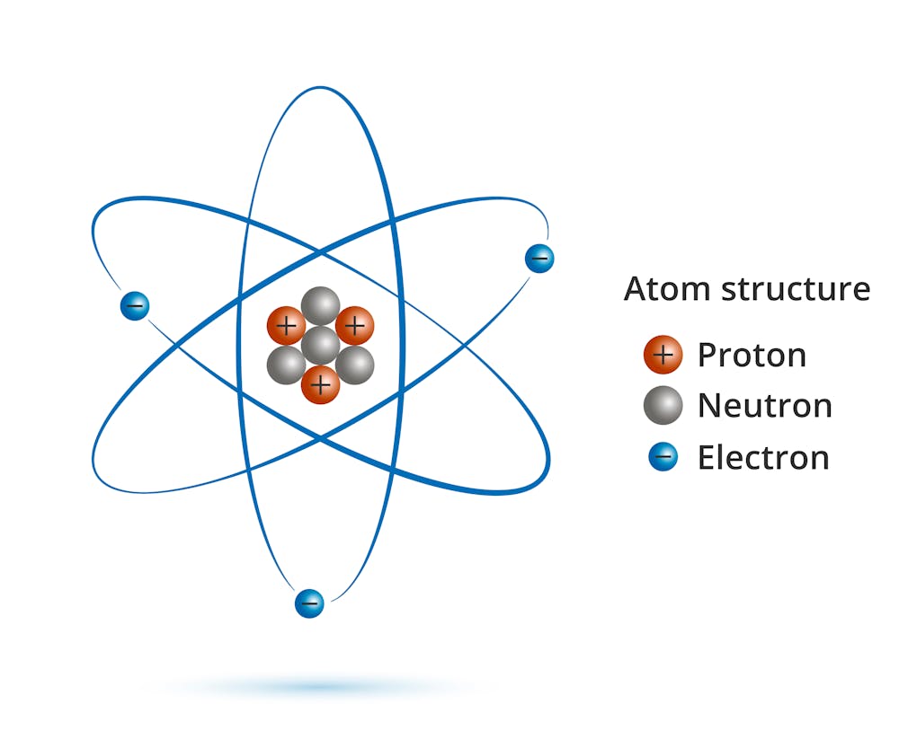
What is the shape of an electron? If you recall pictures from your high school science books, the answer seems quite clear: an electron is a small ball of negative charge that is smaller than an atom. This, however, is quite far from the truth.
Vector FX / Shutterstock.com
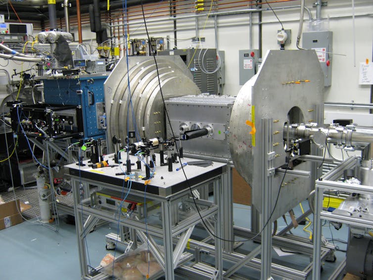
The electron is commonly known as one of the main components of atoms making up the world around us. It is the electrons surrounding the nucleus of every atom that determine how chemical reactions proceed. Their uses in industry are abundant: from electronics and welding to imaging and advanced particle accelerators. Recently, however, a physics experiment called Advanced Cold Molecule Electron EDM (ACME) put an electron on the center stage of scientific inquiry. The question that the ACME collaboration tried to address was deceptively simple: What is the shape of an electron?
Classical and quantum shapes?
As far as physicists currently know, electrons have no internal structure – and thus no shape in the classical meaning of this word. In the modern language of particle physics, which tackles the behavior of objects smaller than an atomic nucleus, the fundamental blocks of matter are continuous fluid-like substances known as “quantum fields” that permeate the whole space around us. In this language, an electron is perceived as a quantum, or a particle, of the “electron field.” Knowing this, does it even make sense to talk about an electron’s shape if we cannot see it directly in a microscope – or any other optical device for that matter?
To answer this question we must adapt our definition of shape so it can be used at incredibly small distances, or in other words, in the realm of quantum physics. Seeing different shapes in our macroscopic world really means detecting, with our eyes, the rays of light bouncing off different objects around us.
Simply put, we define shapes by seeing how objects react when we shine light onto them. While this might be a weird way to think about the shapes, it becomes very useful in the subatomic world of quantum particles. It gives us a way to define an electron’s properties such that they mimic how we describe shapes in the classical world.
What replaces the concept of shape in the micro world? Since light is nothing but a combination of oscillating electric and magnetic fields, it would be useful to define quantum properties of an electron that carry information about how it responds to applied electric and magnetic fields. Let’s do that.
Harvard Department of Physics, CC BY-NC-SA
Electrons in electric and magnetic fields
As an example, consider the simplest property of an electron: its electric charge. It describes the force – and ultimately, the acceleration the electron would experience – if placed in some external electric field. A similar reaction would be expected from a negatively charged marble – hence the “charged ball” analogy of an electron that is in elementary physics books. This property of an electron – its charge – survives in the quantum world.
Likewise, another “surviving” property of an electron is called the magnetic dipole moment. It tells us how an electron would react to a magnetic field. In this respect, an electron behaves just like a tiny bar magnet, trying to orient itself along the direction of the magnetic field. While it is important to remember not to take those analogies too far, they do help us see why physicists are interested in measuring those quantum properties as accurately as possible.
What quantum property describes the electron’s shape? There are, in fact, several of them. The simplest – and the most useful for physicists – is the one called the electric dipole moment, or EDM.
In classical physics, EDM arises when there is a spatial separation of charges. An electrically charged sphere, which has no separation of charges, has an EDM of zero. But imagine a dumbbell whose weights are oppositely charged, with one side positive and the other negative. In the macroscopic world, this dumbbell would have a non-zero electric dipole moment. If the shape of an object reflects the distribution of its electric charge, it would also imply that the object’s shape would have to be different from spherical. Thus, naively, the EDM would quantify the “dumbbellness” of a macroscopic object.
Electric dipole moment in the quantum world
The story of EDM, however, is very different in the quantum world. There the vacuum around an electron is not empty and still. Rather it is populated by various subatomic particles zapping into virtual existence for short periods of time.
Designua/Shutterstock.com
These virtual particles form a “cloud” around an electron. If we shine light onto the electron, some of the light could bounce off the virtual particles in the cloud instead of the electron itself.
This would change the numerical values of the electron’s charge and magnetic and electric dipole moments. Performing very accurate measurements of those quantum properties would tell us how these elusive virtual particles behave when they interact with the electron and if they alter the electron’s EDM.
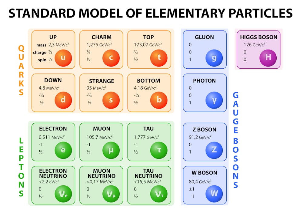
Most intriguing, among those virtual particles there could be new, unknown species of particles that we have not yet encountered. To see their effect on the electron’s electric dipole moment, we need to compare the result of the measurement to theoretical predictions of the size of the EDM calculated in the currently accepted theory of the Universe, the Standard Model.
So far, the Standard Model accurately described all laboratory measurements that have ever been performed. Yet, it is unable to address many of the most fundamental questions, such as why matter dominates over antimatter throughout the universe. The Standard Model makes a prediction for the electron’s EDM too: it requires it to be so small that ACME would have had no chance of measuring it. But what would have happened if ACME actually detected a non-zero value for the electric dipole moment of the electron?

AP Photo/KEYSTONE/Martial Trezzini
Patching the holes in the Standard Model
Theoretical models have been proposed that fix shortcomings of the Standard Model, predicting the existence of new heavy particles. These models may fill in the gaps in our understanding of the universe. To verify such models we need to prove the existence of those new heavy particles. This could be done through large experiments, such as those at the international Large Hadron Collider (LHC) by directly producing new particles in high-energy collisions.
Alternatively, we could see how those new particles alter the charge distribution in the “cloud” and their effect on electron’s EDM. Thus, unambiguous observation of electron’s dipole moment in ACME experiment would prove that new particles are in fact present. That was the goal of the ACME experiment.
This is the reason why a recent article in Nature about the electron caught my attention. Theorists like myself use the results of the measurements of electron’s EDM – along with other measurements of properties of other elementary particles – to help to identify the new particles and make predictions of how they can be better studied. This is done to clarify the role of such particles in our current understanding of the universe.
What should be done to measure the electric dipole moment? We need to find a source of very strong electric field to test an electron’s reaction. One possible source of such fields can be found inside molecules such as thorium monoxide. This is the molecule that ACME used in their experiment. Shining carefully tuned lasers at these molecules, a reading of an electron’s electric dipole moment could be obtained, provided it is not too small.
However, as it turned out, it is. Physicists of the ACME collaboration did not observe the electric dipole moment of an electron – which suggests that its value is too small for their experimental apparatus to detect. This fact has important implications for our understanding of what we could expect from the Large Hadron Collider experiments in the future.
Interestingly, the fact that the ACME collaboration did not observe an EDM actually rules out the existence of heavy new particles that could have been easiest to detect at the LHC. This is a remarkable result for a tabletop-sized experiment that affects both how we would plan direct searches for new particles at the giant Large Hadron Collider, and how we construct theories that describe nature. It is quite amazing that studying something as small as an electron could tell us a lot about the universe.
Alexey Petrov, Professor of Physics, Wayne State University
This article is republished from The Conversation under a Creative Commons license. Read the original article.
![]()
Rapid-response (non-linear) teaching: report January 25, 2018
Posted by apetrov in Blogroll, Education, Near Physics, Physics, Science.Tags: non-linear teaching, rapid-response teaching
add a comment
Some of you might remember my previous post about non-linear teaching, where I described a new teaching strategy that I came up with and was about to implement in teaching my undergraduate Classical Mechanics I class. Here I want to report on the outcomes of this experiment and share some of my impressions on teaching.
Course description
Our Classical Mechanics class is a gateway class for our physics majors. It is the first class they take after they are done with general physics lectures. So the students are already familiar with the (simpler version of the) material they are going to be taught. The goal of this class is to start molding physicists out of physics students. It is a rather small class (max allowed enrollment is 20 students; I had 22 in my class), which makes professor-student interaction rather easy.
Rapid-response (non-linear) teaching: generalities
To motivate the method that I proposed, I looked at some studies in experimental psychology, in particular in memory and learning studies. What I was curious about is how much is currently known about the process of learning and what suggestions I can take from the psychologists who know something about the way our brain works in retaining the knowledge we receive.
As it turns out, there are some studies on this subject (I have references, if you are interested). The earliest ones go back to 1880’s when German psychologist Hermann Ebbinghaus hypothesized the way our brain retains information over time. The “forgetting curve” that he introduced gives approximate representation of information retention as a function of time. His studies have been replicated with similar conclusions in recent experiments.
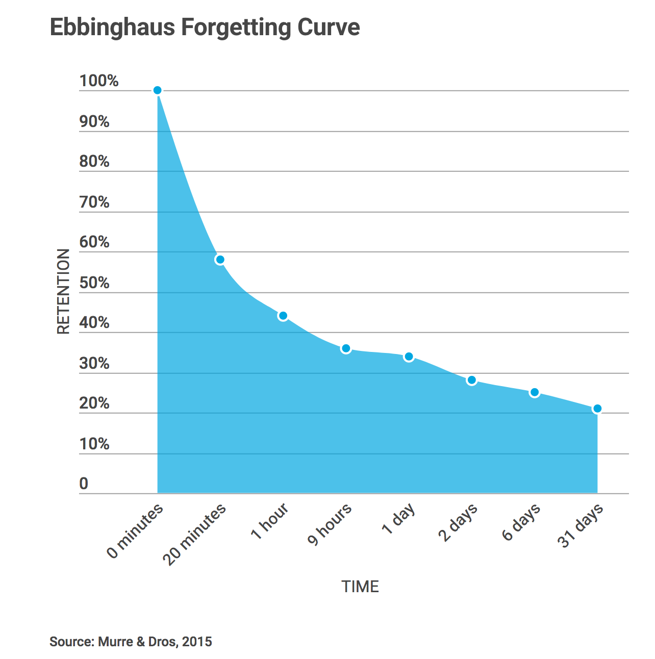 The upshot of these studies is that loss of learned information is pretty much exponential; as can be seen from the figure on the left, in about a day we only retain about 40% of what we learned.
Psychologists also learned that one of the ways to overcome the loss of information is to (meaningfully) retrieve it: this is how learning happens. Retrieval is critical for robust, durable, and long-term learning. It appears that every time we retrieve learned information, it becomes more accessible in the future. It is, however, important how we retrieve that stored information: simple re-reading of notes or looking through the examples will not be as effective as re-working the lecture material. It is also important how often we retrieve the stored info.
So, here is what I decided to change in the way I teach my class in light of the above-mentioned information (no pun intended).
Rapid-response (non-linear) teaching: details
To counter the single-day information loss, I changed the way homework is assigned: instead of assigning homework sets with 3-4-5 problems per week, I introduced two types of homework assignments: short homeworks and projects.
Short homework assignments are single-problem assignments given after each class that must be done by the next class. They are designed such that a student needs to re-derive material that was discussed previously in class (with small new twist added). For example, if the block-down-to-incline problem was discussed in class, the short assignment asks to redo the problem with a different choice of coordinate axes. This way, instead of doing an assignment in the last minute at the end of the week, the students are forced to work out what they just learned in class every day (meaningful retrieval)!
The second type of assignments, project homework assignments are designed to develop understanding of how topics in a given chapter relate to each other. There are as many project assignments as there are chapters. Students get two weeks to complete them.
At the end, the students get to solve approximately the same number of problems over the course of the semester.
For a professor, the introduction of short homework assignments changes the way class material is presented. Depending on how students performed on the previous short homework, I adjusted the material (both speed and volume) that we discussed in class. I also designed examples for the future sections in such a way that I could repeat parts of the topic that posed some difficulties in comprehension. Overall, instead of a usual “linear” propagation of the course, we moved along something akin to helical motion, returning and spending more time on topics that students found more difficult (hence “rapid-response or non-linear” teaching).
Other things were easy to introduce: for instance, using Socrates’ method in doing examples. The lecture itself was an open discussion between the prof and students.
Outcomes
So, I have implemented this method in teaching Classical Mechanics I class in Fall 2017 semester. It was not an easy exercise, mostly because it was the first time I was teaching 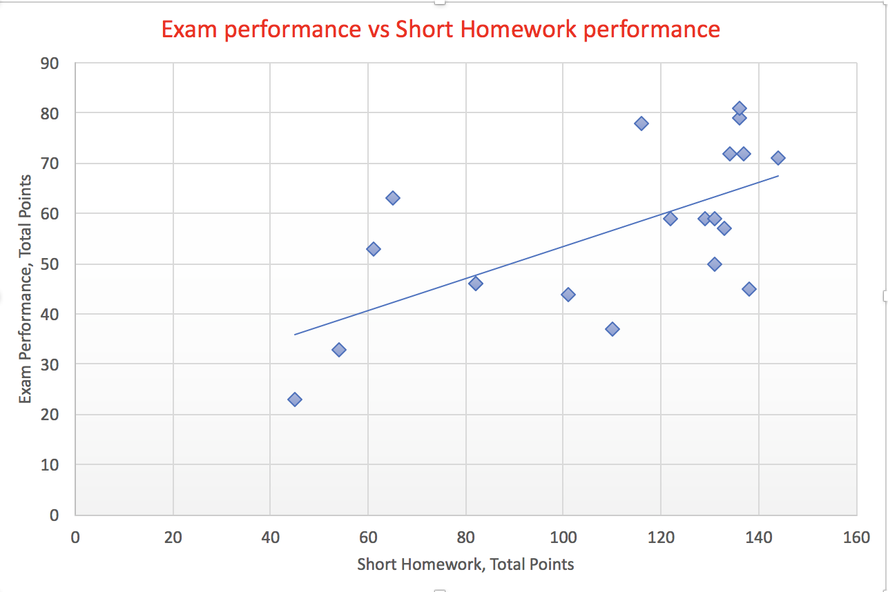 this class and had no grader help. I would say the results confirmed my expectations: introduction of short homework assignments helps students to perform better on the exams. Now, my statistics is still limited: I only had 20 students in my class. Yet, among students there were several who decided to either largely ignore short homework assignments or did them irregularly. They were given zero points for each missed short assignment. All students generally did well on their project assignments, yet there appears some correlation (see graph above) between the total number of points acquired on short homework assignments and exam performance (measured by a total score on the Final and two midterms). This makes me thing that short assignments were beneficial for students. I plan to teach this course again next year, which will increase my statistics.
I was quite surprised that my students generally liked this way of teaching. In fact, they were disappointed that I decided not to apply this method for the Mechanics II class that I am teaching this semester. They also found that problems assigned in projects were considerably harder than the problems from the short assignments (this is how it was supposed to be).
For me, this was not an easy semester. I had to develop my set of lectures — so big thanks go to my colleagues Joern Putschke and Rob Harr who made their notes available. I spent a lot of time preparing this course, which, I think, affected my research outcome last semester. Yet, most difficulties are mainly Wayne State-specifics: Wayne State does not provide TAs for small classes, so I had to not only design all homework assignments, but also grade them (on top of developing the lectures from the ground up). During the semester, it was important to grade short assignments in the same day I received them to re-tune lectures, this did take a lot of my time. I would say TAs would certainly help to run this course — so I’ll be applying for some internal WSU educational grants to continue development of this method. I plan to employ it again next year to teach Classical Mechanics.
Non-linear teaching October 9, 2017
Posted by apetrov in Blogroll, Physics, Science.3 comments
I wanted to share some ideas about a teaching method I am trying to develop and implement this semester. Please let me know if you’ve heard of someone doing something similar.
This semester I am teaching our undergraduate mechanics class. This is the first time I am teaching it, so I started looking into a possibility to shake things up and maybe apply some new method of teaching. And there are plenty offered: flipped classroom, peer instruction, Just-in-Time teaching, etc. They all look to “move away from the inefficient old model” where there the professor is lecturing and students are taking notes. I have things to say about that, but not in this post. It suffices to say that most of those approaches are essentially trying to make students work (both with the lecturer and their peers) in class and outside of it. At the same time those methods attempt to “compartmentalize teaching” i.e. make large classes “smaller” by bringing up each individual student’s contribution to class activities (by using “clickers”, small discussion groups, etc). For several reasons those approaches did not fit my goal this semester.
Our Classical Mechanics class is a gateway class for our physics majors. It is the first class they take after they are done with general physics lectures. So the students are already familiar with the (simpler version of the) material they are going to be taught. The goal of this class is to start molding physicists out of students: they learn to simplify problems so physics methods can be properly applied (that’s how “a Ford Mustang improperly parked at the top of the icy hill slides down…” turns into “a block slides down the incline…”), learn to always derive the final formula before plugging in numbers, look at the asymptotics of their solutions as a way to see if the solution makes sense, and many other wonderful things.
So with all that I started doing something I’d like to call non-linear teaching. The gist of it is as follows. I give a lecture (and don’t get me wrong, I do make my students talk and work: I ask questions, we do “duels” (students argue different sides of a question), etc — all of that can be done efficiently in a class of 20 students). But instead of one homework with 3-4 problems per week I have two types of homework assignments for them: short homeworks and projects.
Short homework assignments are single-problem assignments given after each class that must be done by the next class. They are designed such that a student need to re-derive material that we discussed previously in class with small new twist added. For example, in the block-down-to-incline problem discussed in class I ask them to choose coordinate axes in a different way and prove that the result is independent of the choice of the coordinate system. Or ask them to find at which angle one should throw a stone to get the maximal possible range (including air resistance), etc. This way, instead of doing an assignment in the last minute at the end of the week, students have to work out what they just learned in class every day! More importantly, I get to change how I teach. Depending on how they did on the previous short homework, I adjust the material (both speed and volume) discussed in class. I also design examples for the future sections in such a way that I can repeat parts of the topic that was hard for the students previously. Hence, instead of a linear propagation of the course, we are moving along something akin to helical motion, returning and spending more time on topics that students find more difficult. That’t why my teaching is “non-linear”.
Project homework assignments are designed to develop understanding of how topics in a given chapter relate to each other. There are as many project assignments as there are chapters. Students get two weeks to complete them.
Overall, students solve exactly the same number of problems they would in a normal lecture class. Yet, those problems are scheduled in a different way. In my way, students are forced to learn by constantly re-working what was just discussed in a lecture. And for me, I can quickly react (by adjusting lecture material and speed) using constant feedback I get from students in the form of short homeworks. Win-win!
I will do benchmarking at the end of the class by comparing my class performance to aggregate data from previous years. I’ll report on it later. But for now I would be interested to hear your comments!
Nobel week 2015 October 5, 2015
Posted by apetrov in Blogroll, Physics, Science.Tags: physics, precision measurements
1 comment so far
So, once again, the Nobel week is upon us. And one of the topics of conversations for the “water cooler chat” in physics departments around the world is speculations on who (besides the infamous Hungarian “physicist” — sorry for the insider joke, I can elaborate on that if asked) would get the Nobel Prize in physics this year. What is your prediction?
With invention of various metrics for “measuring scientific performance” one can make educated guesses — and even put predictions on the industrial footage — see Thomson Reuters predictions based on a number of citations (they did get the Englert-Higgs prize right, but are almost always off). Or even try your luck with on-line betting (sorry, no link here — I don’t encourage this). So there is a variety of ways to make you interested.
My predictions for 2015: Vera Rubin for Dark Matter or Deborah Jin for fermionic condensates. But you must remember that my record is no better than that of Thomson Reuters.
So, you want to go on sabbatical… February 5, 2015
Posted by apetrov in Blogroll, Near Physics, Physics, Science.add a comment
Every seven years or so a professor in a US/Canadian University can apply for a sabbatical leave. It’s a very nice thing: your University allows you to catch up on your research, learn new techniques, write a book, etc. That is to say, you become a postdoc again. And in many cases questions arise: should I stay at my University or go somewhere else? In many cases yearlong sabbaticals are not funded by the home University, i.e. you have to find additional sources of funding to keep your salary.
I am on a year-long sabbatical this academic year. So I had to find a way to fund my sabbatical (my University only pays 60% of my salary). I spent Fall 2014 semester at Fermilab and am spending Winter 2015 semester at the University of Michigan, Ann Arbor.
Here are some helpful resources for those who are looking to fund their sabbatical next year. As you could see from the list, they are slightly tilted towards theoretical physics. Yet, there are many resources that are useful for any profession. Of course your success depends on many factors: whether or not you would like to stay in the US or go abroad, competition, etc.
- General resources:
Guggenheim Foundation
Deadline: September
Fulbright Scholar Program
Deadline: August
- USA/Canada:
Simons Fellowship
Deadline: September
IAS Princeton (Member/Sabbatical)
Deadline: November
Perimeter Institute:
Visitors
Visiting Professors
Deadline: November
Radcliffe Institute at Harvard University
Deadline: November
FNAL:
URA Visiting Scholar program
Intensity Frontier Fellowships
Deadline: twice a year
- Europe:
Alexander von Humbuldt:
Friedrich Wilhelm Bessel Research Award
Humboldt Research Award
Deadline: varies
Marie Curie International Incoming Fellowships
Deadline: varies
CERN Short Term visitors
Deadline: varies
Hans Fischer Senior Fellowship (TUM-IAS, Munchen)
Deadline: varies
Some general info that could also be useful can be found here.
I don’t pretend to have a complete list, but those sites were useful for me. I did not apply to all of those programs — and rather unfortunately, missed a deadline for the Simons Fellowship. Many University also have separate funds for sabbatical visitors. So if there is a University one wants to visit, it’s best to ask.
On a final note, it might be useful to be prepared and figure out, if you get funded, how the money/fellowship will find a way to your University and to you. Also, in many cases “60% of the salary” paid by your University while you are on a sabbatical leave means that you would have to find not only the remaining 40% of your salary, but also fringes that your University would take from your fellowship. So the amount that you’d need to find is more than 40% of your salary. Please don’t make a mistake that I made. 🙂
Good luck!
And the 2013 Nobel Prize in Physics goes to… October 8, 2013
Posted by apetrov in Particle Physics, Physics, Science, Uncategorized.1 comment so far
Today the 2013 Nobel Prize in Physics was awarded to François Englert (Université Libre de Bruxelles, Belgium) and Peter W. Higgs (University of Edinburgh, UK). The official citation is “for the theoretical discovery of a mechanism that contributes to our understanding of the origin of mass of subatomic particles, and which recently was confirmed through the discovery of the predicted fundamental particle, by the ATLAS and CMS experiments at CERN’s Large Hadron Collider.” What did they do almost 50 years ago that warranted their Nobel Prize today? Let’s see (for the simple analogy see my previous post from yesterday).
The overriding principle of building a theory of elementary particle interactions is symmetry. A theory must be invariant under a set of space-time symmetries (such as rotations, boosts), as well as under a set of “internal” symmetries, the ones that are specified by the model builder. This set of symmetries restrict how particles interact and also puts constraints on the properties of those particles. In particular, the symmetries of the Standard Model of particle physics require that W and Z bosons (particles that mediate weak interactions) must be massless. Since we know they must be massive, a new mechanism that generates those masses (i.e. breaks the symmetry) must be put in place. Note that a theory with massive W’s and Z that are “put in theory by hand” is not consistent (renormalizable).
The appropriate mechanism was known in the beginning of the 1960’s. It goes under the name of spontaneous symmetry breaking. In one variant it involves a spin-zero field whose self-interactions are governed by a “Mexican hat”-shaped potential
 It is postulated that the theory ends up in vacuum state that “breaks” the original symmetries of the model (like the valley in the picture above). One problem with this idea was that a theorem by G. Goldstone required a presence of a massless spin-zero particle, which was not experimentally observed. It was Robert Brout, François Englert, Peter Higgs, and somewhat later (but independently), by Gerry Guralnik, C. R. Hagen, Tom Kibble who showed a loophole in a version of Goldstone theorem when it is applied to relativistic gauge theories. In the proposed mechanism massless spin-zero particle does not show up, but gets “eaten” by the massless vector bosons giving them a mass. Precisely as needed for the electroweak bosons W and Z to get their masses! A massive particle, the Higgs boson, is a consequence of this (BEH or Englert-Brout-Higgs-Guralnik-Hagen-Kibble) mechanism and represents excitation of the Higgs field about its new vacuum state.
It took about 50 years to experimentally confirm the idea by finding the Higgs boson! Tracking the historic timeline, the first paper by Englert and Brout, was sent to Physical Review Letter on 26 June 1964 and published in the issue dated 31 August 1964. Higgs’ paper, received by Physical Review Letters on 31 August 1964 (on the same day Englert and Brout’s paper was published) and published in the issue dated 19 October 1964. What is interesting is that the original version of the paper by Higgs, submitted to the journal Physics Letters, was rejected (on the grounds that it did not warrant rapid publication). Higgs revised the paper and resubmitted it to Physical Review Letters, where it was published after another revision in which he actually pointed out the possibility of the spin-zero particle — the one that now carries his name. CERN’s announcement of Higgs boson discovery came 4 July 2012.
Is this the last Nobel Prize for particle physics? I think not. There are still many unanswered questions — and the answers would warrant Nobel Prizes. Theory of strong interactions (which ARE responsible for masses of all luminous matter in the Universe) is not yet solved analytically, the nature of dark matter is not known, the picture of how the Universe came to have baryon asymmetry is not cleared. Is there new physics beyond what we already know? And if yes, what is it? These are very interesting questions that need answers.
Higgs mechanism for electrical engineers October 7, 2013
Posted by apetrov in Particle Physics, Physics, Science, Uncategorized.Tags: higgs boson
2 comments
Since the Higgs boson’s discovery a little over a year ago at CERN I have been getting a lot of questions from my friends to explain to them “what this Higgs thing does.” So I often tried to use the crowd analogy that is ascribed to Prof. David Miller, to describe the Higgs (or Englert-Brout-Higgs-Guralnik-Hagen-Kibble) mechanism. Interestingly enough, it did not work well for most of my old school friends, majority of whom happen to pursue careers in engineering. So I thought that perhaps another analogy would be more appropriate. Here it is, please let me know what you think!
Imagine Higgs field as represented by some quantity of slightly magnetized iron filings, i.e. small pieces of iron that look like powder, spread over a table or other surface to represent Higgs field that permeates the Universe. Iron filings are common not only as dirt in metal shops, they are often used in school experiments and other science demonstrations to visualize the magnetic field. It is important for them to be slightly magnetized, as this represents self-interaction of the Higgs field. Here they are pictured in a somewhat cartoonish way:
 How can Higgs field generate mass? Moreover, how can one field generate different masses for different types of particles? Let us first make an analogue of fermion mass generation. If we take a small magnet and put it in the filings, the magnet would pick up a bunch of filings, right? How much would it pick up? It depends on the “strength” of that magnet. It could be a little:

…or it could be a lot, depending on what kind of magnet we use — or how strong it is:

If we neglect the masses of our magnets, as we assumed they are small, the mass of the picked up mess with the magnets inside is totally determined by the mass of the picked filings, which in turn is determined by the interaction strength between the magnets and the filings. This is precisely how fermion mass generation works in the Standard Model!
In the Standard Model the massless fermions are coupled to the Higgs field via so-called Yukawa interactions, whose strength is parametrized by a number, the Yukawa coupling constant. For different fermion types (or flavors) the couplings would be numerically different, ranging from one to one part in a million. As a result of interaction with the Higgs field (NOT the boson!) in the form of its vacuum expectation value, all fermions acquire masses (ok, maybe not all — neutrinos could be different). And those masses would depend on the strength of the interaction of fermions with Higgs field, just like in our example with magnets and iron filings!
Now imagine that we simply kicked the table! No magnets. The filings would clamp together to form lumps of filings. Each lump would have a mass, which would only depend on how strong the filings attract to each other (remember that they are slightly magnetized?). If we don’t know how strong they are magnetized, we cannot tell how massive each lamp will be, so we would have to measure their masses.
 This gives a good analogy of the fact that Higgs boson is an excitation of the Higgs field (the fact that was pointed out by Higgs), and why we cannot predict its mass from the first principles, but need a direct observation at the LHC!
Notice that this picture (so far) does not provide direct analogy to how gauge bosons (W’s and Z bosons) receive their masses. W’s and Z are also initially massless because of the gauge (internal) symmetries required by the construction of the Standard Model. We did know their mass from earlier CERN and SLAC experiments — and even prior to those, we knew that W’s were massive from the fact that weak interactions are of the finite range.
To extend our analogy, let’s clean up the mess — literally! Let’s throw a bucket of water over the table covered with those iron filings and see what happens. Streams of water would pick up iron filings and flow from the table. Assuming that that water’s mass is negligible, the total mass of those water streams (aka dirty water) would be completely determined by the mass of picked iron filings, just like masses of W’s and Z are determined by the Higgs field.
This explanation seemed to work better for my engineering friends! What do you think?
